Rkf45
A 4 (5) order Runge-Kutta-Fehlberg solver (Dormand & Prince Pair) for non-stiff intial value problem (IVP)
Syntax for 1st-Order IVP
rkf45(dydt, t_start, t_end, nstep, y0) |
Input: dydt is a user defined function of the form dydt(t, y) => {some expression of y and t} t_start is a real number for initial time t_end is a real number of end time nstep is an positive integer implies the preferred time steps for the solutions y0 is a real number for the initial value of y when t = t_start Result: A row vector gives the time points of t for the solutions A column vector gives the solutions y for the time points t. |
rkf45(dydt, t_start, t_end, nstep, y0, abserr, relerr) |
Input: dydt is a user defined function of the form dydt(y, t) => {some expression of y and t} t_start is a real number for initial time t_end is a real number of end time nstep is an positive integer implies the preferred time steps for the solutions y0 is a real number for the initial value of y when t = t_start abserr is a real number for absolute tolerance relerr is a real number for relative tolerance Result: A row vector gives the time points of t for the solutions A column vector gives the solutions y for the time points t. |
rkf45(dydt, t, y0) |
Input: dydt is a user defined function of the form dydt(y, t) => {some expression of y and t} t is a row/column vector which gives the preferred time points for the solutions y0 is a real number for the initial value of y when t = t[0] Result: A row vector gives the time points of t for the solutions A column vector gives the solutions y for the time points t. |
rkf45(dydt, t, y0, abserr, relerr) |
Input: dydt is a user defined function of the form dydt(y, t) => {some expression of y and t} t is a row/column vector which gives the preferred time points for the solutions y0 is a real number for the initial value of y when t = t[0] abserr is a real number for absolute tolerance relerr is a real number for relative tolerance Result: A row vector gives the time points of t for the solutions A column vector gives the solutions y for the time points t. |
Example I
Solve Problem
y'=0.25*y*(1-y/20)
y(0) = 1
between the time [0,20].
Input |
Output |
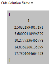
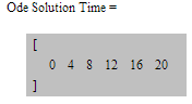
dydt(t, y) => 0.25*y*(1-y/20) rkf45(dydt, 0, 20, 5, 1) |
|
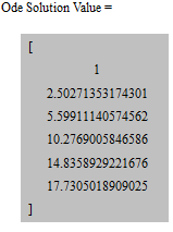
dydt(t, y) => 0.25*y*(1-y/20) rkf45(dydt, 0, 20, 5, 1, 1.0e-10, 1.0e-10) |
|
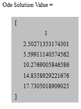
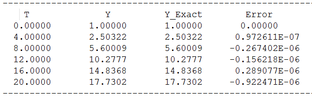
dydt(t, y) => 0.25*y*(1-y/20) t=[0, 4, 8, 12, 16, 20] rkf45(dydt, t, 1) |
|
dydt(t, y) => 0.25*y*(1-y/20) t=[0, 4, 8, 12, 16, 20] rkf45(dydt, t, 1, 1.0e-10, 1.0e-10) |
|
Discussion:
Problem has an exact solution of y(t) = 20.0 / ( 1.0 + 19.0 * exp ( - 0.25 * t ) )
Compare the numerical solution above with the exact solution you get
Syntax for High-Order IVP
rkf45(<dy1dt, ...>, t_start, t_end, nstep, y0) |
Input: <dy1dt, dy2dt, ...> is a group of user defined functions of the form dydt(t, y1, y2, ...) => {some expression of t, y1, y2, ...}, which are enclosed with '<>'. These functions defined the all 1st-order IVP differential equations converted from the high-order ODE. t_start is a real number for initial time t_end is a real number of end time nstep is an positive integer implies the preferred time steps for the solutions y0 is a real number for the initial value of y when t = t_start Result: A row vector gives the time points of t for the solutions A matrix gives the solutions y for the time points t whose first column is solution for y1, second row for y2, etc. |
rkf45(<dy1dt, ...>, t_start, t_end, nstep, y0, abserr, relerr) |
Input: <dy1dt, dy2dt, ...> is a group of user defined functions of the form dydt(t, y1, y2, ...) => {some expression of t, y1, y2, ...}, which are enclosed with '<>'.These functions defined the all 1st-order IVP differential equations converted from the high-order ODE. t_start is a real number for initial time t_end is a real number of end time nstep is an positive integer implies the preferred time steps for the solutions y0 is a real number for the initial value of y when t = t_start abserr is a real number for absolute tolerance relerr is a real number for relative tolerance Result: A row vector gives the time points of t for the solutions A matrix gives the solutions y for the time points t whose first column is solution for y1, second row for y2, etc. |
rkf45(<dy1dt, ...>, t, y0) |
Input: <dy1dt, dy2dt, ...> is a group of user defined functions of the form dydt(t, y1, y2, ...) => {some expression of t, y1, y2, ...}, which are enclosed with '<>'. These functions defined the all 1st-order IVP differential equations converted from the high-order ODE. t is a row/column vector which gives the preferred time points for the solutions y0 is a real number for the initial value of y when t = t[0] Result: A row vector gives the time points of t for the solutions A matrix gives the solutions y for the time points t whose first column is solution for y1, second row for y2, etc. |
rkf45(<dy1dt, ...>, t, y0, abserr, relerr) |
Input: <dy1dt, dy2dt, ...> is a group of user defined functions of the form dydt(t, y1, y2, ...) => {some expression of t, y1, y2, ...}, which are enclosed with '<>'. These functions defined the all 1st-order IVP differential equations converted from the high-order ODE. t is a row/column vector which gives the preferred time points for the solutions y0 is a real number for the initial value of y when t = t[0] abserr is a real number for absolute tolerance relerr is a real number for relative tolerance Result: A row vector gives the time points of t for the solutions A matrix gives the solutions y for the time points t whose first column is solution for y1, second row for y2, etc. |
Example 2
Solve Problem
y''+ y = 0
y(0) = 1; y'(0) = 0;
between the time [0, 2π].
The above 2nd order ODE can be rewritten to a group of two 1st order ODE
y1' = y2
y2' = -y1
y1(0) = 1; y2(0) = 0;
Input |
Output |
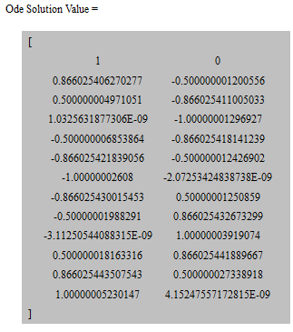
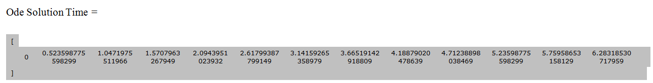
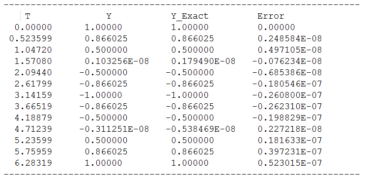
dy1dt(t, y1, y2) => y2 dy2dt(t, y1, y2) => - y1 rkf45(<dy1dt, dy2dt>, 0, 2*Pi, 12, [1, 0]) |
|
Discussion:
Problem has an exact solution of y(t) = cos(t)
Compare the numerical solution above with the exact solution you get
See Also
Created with the Personal Edition of HelpNDoc: Easily create HTML Help documents