Mirk
A solver using 4th order MIRK (mono-implicit Runge-Kutta) scheme for non-stiff or mildly-stiff boundary value problems (BVP)
Syntax:
mirk(<dy1dx, ...>, <bc1, ...>, nlbc, x_a, x_b, nmesh) |
Input: <dy1dx, dy2dx, ...> is a group of user defined functions of the form dydx(x, y1, y2, ...) => {some expression of x, y1, y2, ...}, which are enclosed with '<>'. These functions defined the all 1st-order differential equations from or converted from the BVP ODE. <bc1, bc2, ...> is a group of user defined function of the form bc(y1, y2, ...) => {some expression of y1, y2, ...} which are enclosed with '<>'. These functions define all boundary conditions and they are ordered in a way that the left boundary conditions (at boundary of x = x_a) are written first than all of the right boundary conditions (at boundary x = x_b). Note that for boundary condition like y1(x_a) = a needs to be rewritten as bc1(y1,..) => y1 - a. nlbc is the number of the boundary conditions implemented on the left boundary (where x = x_a) x_a is a real number for the left boundary location x_b is a real number for the right boundary location nmesh is an positive integer implies the preferred mesh grid points for the solutions Result: A row vector gives the mesh points of x for the solutions A matrix gives the solutions y for the mesh points x whose first column is solution for y1, second row for y2, etc. |
mirk(<dy1dx, ...>, <bc1, ...>, nlbc, x_a, x_b, nmesh, torr) |
Input: <dy1dx, dy2dx, ...> is a group of user defined functions of the form dydx(x, y1, y2, ...) => {some expression of x, y1, y2, ...}, which are enclosed with '<>'. These functions defined the all 1st-order differential equations from or converted from the BVP ODE. <bc1, bc2, ...> is a group of user defined function of the form bc(y1, y2, ...) => {some expression of y1, y2, ...} which are enclosed with '<>'. These functions define all boundary conditions and they are ordered in a way that the left boundary conditions (at boundary of x = x_a) are written first than all of the right boundary conditions (at boundary x = x_b). Note that for boundary condition like y1(x_a) = a needs to be rewritten as bc1(y1,..) => y1 - a. nlbc is the number of the boundary conditions implemented on the left boundary (where x = x_a) x_a is a real number for the left boundary location x_b is a real number for the right boundary location nmesh is an positive integer implies the preferred mesh grid points for the solutions torr is a real number for the calculation tolerance Result: A row vector gives the mesh points of x for the solutions A matrix gives the solutions y for the mesh points x whose first column is solution for y1, second row for y2, etc. |
mirk(<dy1dx, ...>, <bc1, ...>, nlbc, x) |
Input: <dy1dx, dy2dx, ...> is a group of user defined functions of the form dydx(x, y1, y2, ...) => {some expression of x, y1, y2, ...}, which are enclosed with '<>'. These functions defined the all 1st-order differential equations from or converted from the BVP ODE. <bc1, bc2, ...> is a group of user defined function of the form bc(y1, y2, ...) => {some expression of y1, y2, ...} which are enclosed with '<>'. These functions define all boundary conditions and they are ordered in a way that the left boundary conditions (at boundary of x = x_a) are written first than all of the right boundary conditions (at boundary x = x_b). Note that for boundary condition like y1(x_a) = a needs to be rewritten as bc1(y1,..) => y1 - a. nlbc is the number of the boundary conditions implemented on the left boundary (where x = x_a) x is a row/column vector which gives the preferred mesh points for the solutions. Note that the first and the last element implies the left and right boundaries. Result: A row vector gives the mesh points of x for the solutions A matrix gives the solutions y for the mesh points x whose first column is solution for y1, second row for y2, etc. |
mirk(<dy1dx, ...>, <bc1, ...>, nlbc, x, torr) |
Input: <dy1dx, dy2dx, ...> is a group of user defined functions of the form dydx(x, y1, y2, ...) => {some expression of x, y1, y2, ...}, which are enclosed with '<>'. These functions defined the all 1st-order differential equations from or converted from the BVP ODE. <bc1, bc2, ...> is a group of user defined function of the form bc(y1, y2, ...) => {some expression of y1, y2, ...} which are enclosed with '<>'. These functions define all boundary conditions and they are ordered in a way that the left boundary conditions (at boundary of x = x_a) are written first than all of the right boundary conditions (at boundary x = x_b). Note that for boundary condition like y1(x_a) = a needs to be rewritten as bc1(y1,..) => y1 - a. nlbc is the number of the boundary conditions implemented on the left boundary (where x = x_a) x is a row/column vector which gives the preferred mesh points for the solutions. Note that the first and the last element implies the left and right boundaries. torr is a real number for the calculation tolerance Result: A row vector gives the mesh points of x for the solutions A matrix gives the solutions y for the mesh points x whose first column is solution for y1, second row for y2, etc. |
Example
Solve Problem
y1' = y2
y2' = 5 * sinh(5 * y1)
with the boundary conditions
y1(0) = 0
y1(1) = 1
Input |
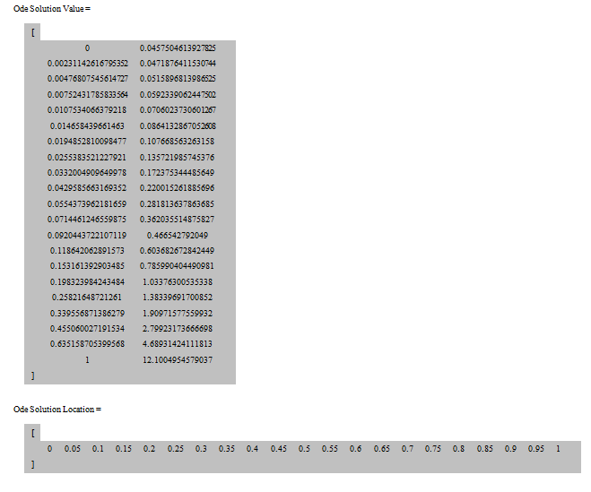
Output |
dy1dx(x, y1, y2) => y2 dy2dx(x, y1, y2) => 5 * sinh(5 * y1) bc1(y1, y2) => y1 bc2(y1, y2) => y1 - 1 mirk(<dy1dx, dy2dx>, <bc1, bc2>, 1, 0, 1, 20) |
|
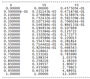
Discussion:
The solution is rewritten in a more friendly way to help to understand:
See Also
Created with the Personal Edition of HelpNDoc: Free EPub and documentation generator